Top Financial Functions in Excel (15+ Functions)

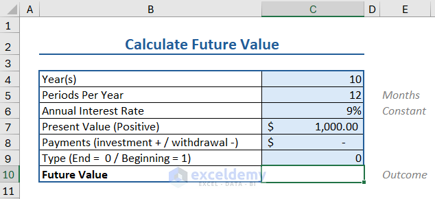
Let’s see an example of how you can apply the FV function to get the future value in Excel. We have the following parameters:

1. Number of years: 10
2. Period value: 12 (as months)
3. Interest rate: 9%
4. Present value: $1000
   Note: This value will be inputted as positive. Important for the calculation (see later).
5. Payment and Type values are left blank (or as 0).

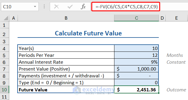
To find the future value, we apply the FV formula as follows:

• C6/C5 calculates the Interest per Period (Annual IR/Periods PY).
• C4*C5 calculates the number of months (Year*Month=Periods).
• Payments (C8) and Type (C9).
• C7 is the Present Value, valued at $1000.
• The negative (-) before the formula plays a crucial role in the calculation.
  • The PV and FV are opposites (PV=Inflow Cash, FV=Outflow Cash)
  • If PV is positive, FV will be negative by calculation.
  • Thus, a negative operator (-) is used to get the correct value.

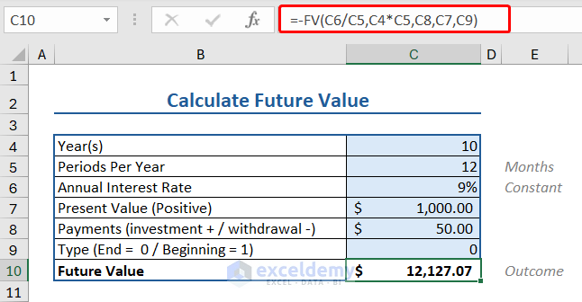
  Let’s say you invest $50 per month. Your account will be valued at $12,127.07

  

  2 – PV Function (Present Value)

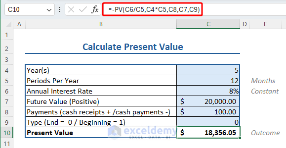
  The PV function is an Excel financial function that calculates the present value of an expected cash flow, which can either be a loan or an investment based on a constant interest rate.

  The syntax of the PV function is:

  PV(rate, nper, pmt, [fv], [type])

  • Rate: It is the rate of interest per period
  • nper: The total number of payment periods in an annuity.
  • pmt: The amount of payment in each period. This amount is fixed. It contains the principal amount and the interest. If pmt is omitted, fv must be included.
  • [fv]: (Optional) It is the future value. Also indicated as the lump sum amount of the present payment.
  • [type]: (Optional) This number is 0 or 1 and indicates when payments are due. 0 at the end of the period and 1 at the beginning.

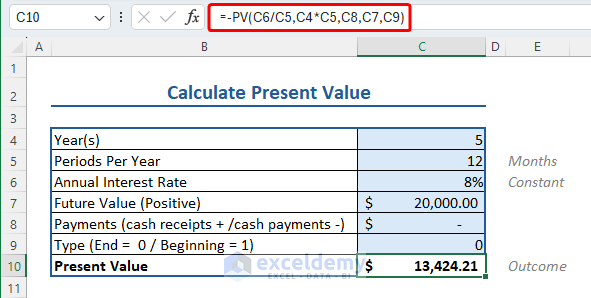
  Let’s see an example of how you can apply the PV function to get the present value of a loan in Excel. We’ll use the following:

  1. Number of years: 5
  2. Period value: 12 (as months)
  3. Interest rate: 8%
  4. Future value: $20000
  5. Payment and Type values are left blank (or as 0).

  Insert the following formula to apply the PV formula to calculate the present value:

  

  • C6/C5 calculates the Interest per Period (Annual IR/Periods PY).
  • C4*C5 calculates the number of months (Year*Month=Periods).
  • Payments (C8) and Type (C9).
  • C7 is the Future Value, valued at $20000.
  • The negative (-) before the formula plays a crucial role in the calculation.
    • The PV and FV are opposites (PV=Inflow Cash, FV=Outflow Cash)
    • If FV is positive, PV will be negative by calculation.
    • Thus a negative operator (-) is used to get the correct value.

    Let’s say you received a cash receipt of $100 per month. Your account will be valued at $18,356.05

    

    3 – PMT Function (Payment)

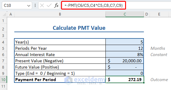
    The PMT function calculates the loan payment for a constant interest rate and constant payment.

    The syntax of the PMT function is:

    PMT(rate, nper, pv, [fv], [type])

    • Rate: It is the rate of interest per period
    • nper: The total number of payment periods.
    • pv: It is the present value. Also indicates the lump sum amount of a future payment.
    • [fv]: (Optional) It is the future value. Also indicated as the lump sum amount of the present payment.
    • [type]: (Optional) This number is 0 or 1 and indicates when payments are due. 0 at the end of the period and 1 at the beginning.

    Let’s apply the PMT function to get the constant payment for a loan at a constant interest rate in Excel. We’ll use the following:

    1. Number of years: 5
    2. Period value: 12 (as months)
    3. Interest rate: 8%
    4. Present value: $20000
    5. Future value and Type values are left blank (or as 0).

    To apply the PMT formula to calculate the payment per period, insert the following formula:

    

    • C6/C5 calculates the Interest per Period (Annual IR/Periods PY).
    • C4*C5 calculates the number of months (Year*Month=Periods).
    • C8 is the Future value, and the Payment Type is C9.
    • C7 is the Present Value, valued at $20000.

    4 – Rate Function (Interest Rate)

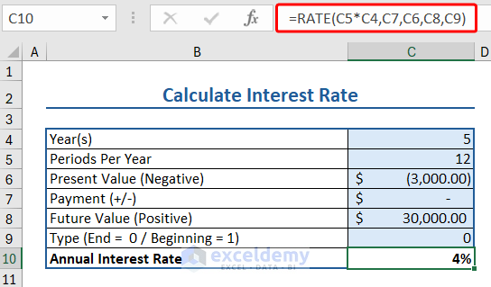
    The RATE function calculates the interest rate per period for an investment or loan.

    The syntax of the RATE function is:

    RATE(nper, pmt, pv, [fv], [type])

    • nper: The total number of payment periods.
    • pmt: The amount of payment in each period. This amount is fixed. It contains the principal amount and the interest. If pmt is omitted, fv must be included.
    • pv: It is the present value. It also indicates the lump sum amount of a future payment.
    • [fv]: (Optional) It is the future value. Also indicated as the lump sum amount of the present payment.
    • [type]: (Optional) This number is 0 or 1 and indicates when payments are due. 0 at the end of the period and 1 at the beginning of the period.

    Let’s apply the RATE function to get the interest rate for a loan for a fixed period of time in Excel. We’ll use the following:

    1. Number of years: 5
    2. Period value: 12 (as months)
    3. Present value: -$3000
    4. Future value: $30000
    5. Payment and Type values are left blank (or as 0).

    To apply the RATE formula to calculate the interest rate, insert the following formula:

    

    • C5*C4 calculates the NPER or number of months (Year*Month=Periods).
    • C4*C5 calculates the number of months (Year*Month=Periods).
    • Payments (C7) and Type (C9).
    • C6 is the Present Value, valued at $3000 and entered as negative as,
      • The PV and FV are opposites (PV=Inflow Cash, FV=Outflow Cash)
      • If PV is positive, FV will be negative by calculation.
      • Thus a negative operator (-) is used to get the correct value.

      5 – NPER Function (Number of Periods)

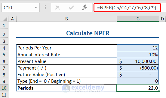
      The financial function NPER calculates period numbers for periodic, constant payments for constant interest rates.

      The syntax of the RATE function is:

      NPER(rate, pmt, pv, [fv], [type])

      • Rate: It is the rate of interest per period
      • pmt: The amount of payment in each period. This amount is fixed. It contains the principal amount and the interest. If pmt is omitted, fv must be included.
      • pv: It is the present value. Also indicated as the lump sum amount of a future payment.
      • [fv]: (Optional) It is the future value. Also indicated as the lump sum amount of the present payment.
      • [type]: (Optional) This number is 0 or 1 and indicates when payments are due. 0 at the end of the period and 1 at the beginning of the period.

      Let’s apply the NPER function to get the number of periods to pay a loan for a fixed interest rate in Excel. We’ll use the following:

      1. Number of years: 12
      2. Annual Interest Rate: 10%
      3. Present value: $10000
      4. Payment: -$500
      5. Future value and Type values are left blank (or as 0).

      Insert the following formula to apply the NPER function to calculate the interest rate:

      

      6 – NPV Function (Net Present Value)

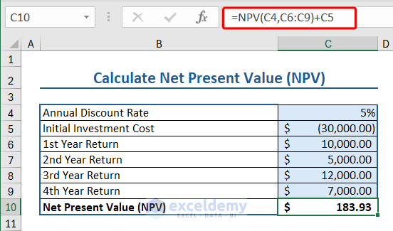
      The NPV function calculates the net present value of an investment.

      The syntax of the NPV function is:

      • Rate: discount rate
      • Value 1, [value2],[value3]…: payments and income. It should be equally spaced in time and occur at the end of each period.

      Let’s use the NPV function to calculate net present value. We’ll use the following:

      • Annual Discount Rate: 5%
      • Initial Investment Cost: $30000
      • 1st Year Return: $10000
      • 2nd Year Return: $5000
      • 3rd Year Return: $12000
      • 4th Year Return: $7000

      Insert the following formula to apply the NPV function to calculate the net present value:

      

      7 – IRR Function (Internal Rate of Return)

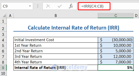
      The IRR function calculates the internal rate of return for a series of cash.

      The syntax of the IRR function is:

      • Values: An array or a reference to cells that contain numbers for which the internal rate of return is calculated
      • [guess]: Guessed number close to the result of IRR.

      Here we have some data relevant to IRR function:

      • Initial Investment Cost: $30000
      • 1st Year Return: $10000
      • 2nd Year Return: $5000
      • 3rd Year Return: $12000
      • 4th Year Return: $7000

      Insert the following formula to apply the IRR formula to calculate the internal rate of return:

      

      8 – XNPV Function (NPV for Non-Scheduled Cash Flow)

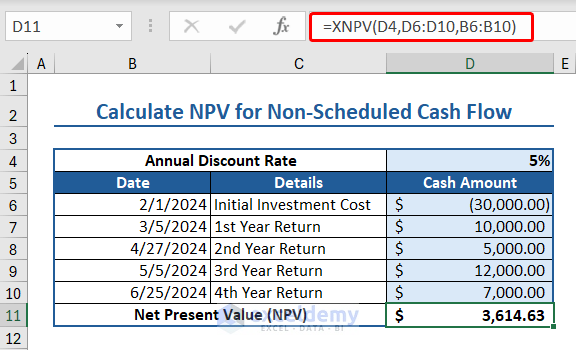
      The XNPV function calculates the net present value of net present value of a cash flow series that are not necessarily periodic.

      The syntax of the XNPV function is:

      XNPV(rate, values, dates)

      • Rate: An array or a reference to cells that contain numbers for which the internal rate of return is calculated
      • Values: A series of cash flows corresponding to a payment schedule (in dates). The first payment is optional and corresponds to a payment that occurs at the beginning of the investment. If the first value is a cost or payment, it must be a negative value. All payments are discounted based on a 365-day year. The values must contain minimum one positive value and one negative value.
      • Dates: A schedule of payment dates that corresponds to the cash flow payments. The first payment date must be in top of the list. But the other dates can occur in any order.

      Here we have some data relevant to XNPV function:

      • Date values arranged in a column.
      • Annual Discount Rate: 5%
      • Initial Investment Cost: $30000
      • 1st Year Return: $10000
      • 2nd Year Return: $5000
      • 3rd Year Return: $12000
      • 4th Year Return: $7000

      Insert the following formula to apply the XNPV function to calculate the net present value for non-scheduled cash flow:

      

      9 – XIRR Function (IRR for Non-Scheduled Cash Flow)

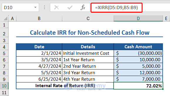
      The XIRR function calculates the internal rate of return for a series of cash flows that occur at irregular intervals.

      The syntax of the XIRR function is:

      XIRR(values, dates, [guess])

      • Values: A series of cash flows corresponding to a payment schedule (in dates). The first payment is optional and corresponds to a payment that occurs at the beginning of the investment. If the first value is a cost or payment, it must be a negative value. All payments are discounted based on a 365-day year. The values must contain minimum one positive value and one negative value.
      • Dates: Payment schedule (in dates). The dates can occur in any order in the list. But dates must be given by using the DATE function.
      • [guess]: A number that is close to the output of XIRR.

      Here we have some data relevant to XIRR function:

      • Date values arranged in a column.
      • Initial Investment Cost: $30000
      • 1st Year Return: $10000
      • 2nd Year Return: $5000
      • 3rd Year Return: $12000
      • 4th Year Return: $7000

      Insert the following formula to apply XIRR formula to calculate the internal rate of return for non-scheduled cash flow:

      

      10 – MIRR Function (Modified Internal Rate of Return)

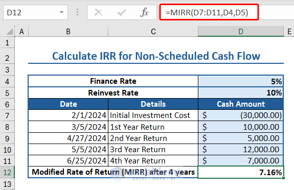
      The MIRR function calculates the modified internal rate of return for a series of periodic cash flows. MIRR considers both the cost of the investment and the reinvestment rate.

      The syntax of the MIRR function is:

      MIRR(values, finance_rate, reinvest_rate)

      • Values: An array or a cell reference that contains cash amount.
      • Finance_rate: The interest rate paid on the money used in the cash flows.
      • Reinvest_rate: The interest rate received on the cash flows after reinvesting them.

      Here we have some data relevant to MIRR function:

      • Finance Rate: 5%
      • Reinvest Rate: 10%
      • Initial Investment Cost: $30000
      • 1st Year Return: $10000
      • 2nd Year Return: $5000
      • 3rd Year Return: $12000
      • 4th Year Return: $7000

      Insert the following formula to apply the MIRR function to calculate the modified internal rate of return after 2 years:

      Insert the following formula to apply the MIRR function to calculate the modified internal rate of return after 4 years:

      

      11 – FVSCHEDULE Function (Future Value Applying Series of Compound Interest Rates)

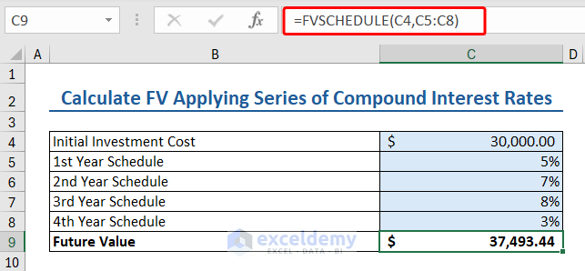
      The FVSCHEDULE function in Excel calculates the future value of an investment based on a schedule of interest rates.

      The syntax of the FVSCHEDULE function:

      • principal: present value
      • schedule: an array of interest rates

      Here we have some data relevant to FVSCHEDULE function:

      • Initial Investment Cost: $30000
      • 1st Year Schedule: 5%
      • 2nd Year Schedule: 7%
      • 3rd Year Schedule: 8%
      • 4th YearSchedule: 3%

      Insert the following formula to apply the FVSCHEDULE function to calculate the future investment value:

      

      12 – PPMT Function (Principal Payment)

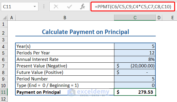
      The PPMT function in Excel calculates the payment on principal for a given period.

      The syntax of the PPMT function:

      PPMT(rate, per, nper, pv, [fv], [type])

      • Rate: Interest rate
      • Per: Period
      • Nper: Number of periods in an annuity.
      • Pv: Present value
      • [fv]: Future value
      • [type]: The number 0 or 1 and indicates when payments are due.

      Here we have some data relevant to PPMT function:

      • Year: 5
      • Periods Per Year: 12
      • Annual Interest Rate: 8%
      • Present Value: $20000
      • Future Value: $ –
      • Period Number: 5
      • Type(End=0/Beginning=1)

      Insert the following formula to apply the PPMT function to calculate the payment on the principal:

      

      13 – RRI Function (Rate of Return)

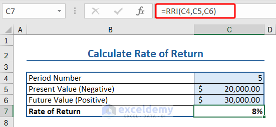
      The RRI function in Excel calculates an equivalent rate of interest for the growth of an investment.

      The syntax of the RRI function:

      Here we have some data relevant to RRI function:

      • Period Number: 5
      • Present Value: $20000
      • Future Value: $30000
      • Rate of Return: 8%

      Insert the following formula to apply the RRI function to calculate the rate of return:

      

      14 – EFFECT Function (Effective Annual Rate of Return)

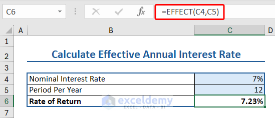
      The EFFECT function in Excel calculates the effective annual rate of interest or rate of return.

      The syntax of the EFFECT function:

      • Nominal_rate: Nominal interest rate
      • Npery: number of compounding periods per year.

      Here we have some data relevant to EFFECT function:

      • Nominal Interest Rate: 7%
      • Period Per Year: 12

      Insert the following formula to apply the EFFECT function to calculate the rate of return:

      

      15 – IPMT Function (Interest Payment)

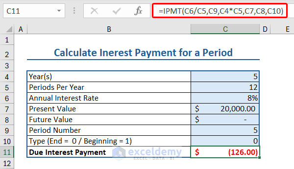
      The IPMT function calculates the due interest payment for a periodic, constant payment and interest rate for a given time period.

      The syntax of the IPMT function is:

      IPMT(rate, per, nper, pv, [fv], [type])

      • Rate: Interest rate
      • Per: Period
      • Nper: Number of periods in an annuity.
      • Pv: Present value
      • [fv]: (Optional)Future value
      • [type]: (Optional) The number 0 or 1 indicates when payments are due.

      Here we have some data relevant to IPMT function:

      • Year: 5
      • Periods Per Year: 12
      • Annual Interest Rate: 8%
      • Present Value: $20000
      • Future Value: $ –
      • Period Number: 5
      • Type(End=0/Beginning=1): 0

      Insert the following formula to apply the IPMT function to calculate the interest payment:

      

      16 – DB Function (Depreciation Value)

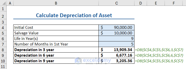
      The DB function calculates the depreciation of any asset using a fixed declining way for a definite time period.

      The syntax of DB function is:

      DB(cost, salvage, life, period, [month])

      • cost: the asset’s initial cost
      • salvage: the asset’s remaining value after the depreciation.
      • life: the number of periods at the end of the depreciating period or the lifetime of an asset when it can be used
      • period: the time period for which you want the depreciation value of the asset. It uses the unit of life.
      • [month]: (Optional) The month number of first year. If it is omitted, then Excel takes it as 12 by default.

      Let us calculate the depreciation value of an asset using DB function. We’ll use the following:

      1. Initial Cost: $90000
      2. Salvage Value: $10000
      3. Life in Years: 9
      4. Number of Months in 1st Year: 5

      We will calculate the depreciation value of the asset after 3, 6, and 9 years.

      To apply the DB function in Excel, insert the following formula in a cell:

      • C4 is the initial cost
      • C5 is salvage value
      • C6 is life
      • 3 is the period till which we want depreciation
      • C7 is the month number in 1st year

      We calculated the depreciation value after 6 and 9 years, as shown in the image below.

      

      17 – STOCKHISTORY Function (Get Stock’s Historical Data)

      The STOCKHISTORY function loads the historical data from a certain period of time regarding a financial instrument (stock) as an array. When this spill formula is applied, Excel dynamically returns the data range in the required amount of cells.

      Note:

      This function is available only for Microsoft 365 Personal, Family, Business Standard, and Business Premium versions
      

      The syntax of STOCKHISTORY function is:

      STOCKHISTORY(stock, start_date, [end_date], [interval], [headers], [property0], [property1], [property2], [property3], [property4], [property5])

      • stock: it is the ticker symbol for the financial instrument of which you want the historical data.
      • start_date: the starting date from which you want the data
      • [end_date]: (Optional) the date till which you want the data
      • [interval]: (Optional) This number denotes the interval of each data. “0” for daily, “1” for weekly, and “2” for monthly interval.
      • [headers]: (Optional) This number is to decide if you want to display headings or not. “0” for no headers, “1” for showing headers, and “2” for showing instrument identifiers and headers.
      • [property0- property5]: (Optional) This number indicates which column from historical data you want to retrieve. “0” for Dates, “1” for Close, “2” for Open, “3” for High, “4” for Low, and “5” for Volume.

      Let’s see how this STOCKHISTORY function works in Excel. We’ll use the following information:

      1. Stock name/Ticker Symbol: Amzn
      2. Start date: 1/1//2024
      3. End Date: 1/20/2024

      Insert the following formula in a cell that has enough blank cells below to place the data fetched using the STOCKHISTORY function:

      • C4 is ticker symbol
      • C5 is start date
      • C6 is end date
      • 0 returns daily data, and 2 retrieves the headers
      • 0 fetches the Dates, and 1 brings the closing amount of the financial instrument